The basics of PID Control
This article aims to help the reader to create a physical perception of the operation of a PID control, without much analysis and mathematical rigor. It intends to introduce the technique to beginners and to improve the knowledge of those already initiated, with the most practical and simplified approach possible.
The basics of PID Control
Some definitions of acronyms and terms used in this article:
- PV: Process variable. Variable that is controlled in the process, such as temperature, pressure, humidity, etc.
- SV or SP: The desired value for the process variable.
- MV: Manipulated variable. Variable on which the controller controls the process, such as the position of a valve, the voltage applied to a heating resistance, etc.
- Error or Deviation: Difference between SV and PV. SV-PV is for reverse action, and PV-SV is for direct action.
- Control action: It can be reverse or direct. It generically defines the action applied to the MV during PV variations.
- Reverse action: If PV increases, MV decreases. Typically used in heating controls.
- Direct action: If PV increases, MV increases. Typically used in refrigeration controls.
The PID control technique consists in calculating an actuation value for the process, using information regarding the desired value and the current value of the process variable. This process actuation value is transformed into a signal suitable for the actuator used (valve, motor, relay) and should ensure stable and precise control.
In a simple way, PID is composed of 3 almost intuitive actions, as shown in the following table:
| P | PROPORTIONAL CORRECTION TO THE ERROR | The correction to be applied to the process must increase in proportion to the progression of the error between the current and the desired value. |
| I | PROPORTIONAL CORRECTION TO THE PRODUCT ERROR x TIME | Small errors, but ones that have existed for a long time, require more intensive correction. |
| D | PROPORTIONAL CORRECTION TO THE ERROR RATE OF CHANGE | If the error is varying too fast, this rate of change must be reduced to avoid oscillations. |
N20K48 is the process and temperature controller with the highest sampling rate in 2024.
A little bit of mathematics
The most usual PID equation is as follows:
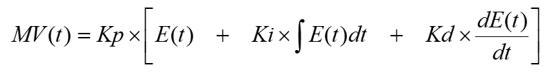
Where Kp, Ki, and Kd are the gains of the P, I, and D parts and define the intensity of each action.
PID devices from different manufacturers implement this equation in different ways. It is usual to adopt the concept of “Proportional Band” instead of Kp, “Derivative Time” instead of Kd, and “Integral Rate” or “Reset” instead of Ki, leaving the equation as follows:
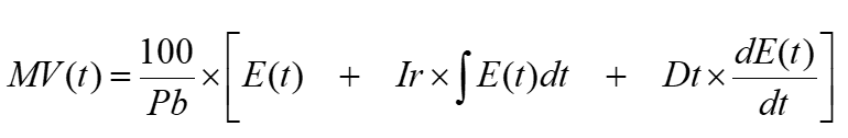
Where Pb, Ir, and Dt are related to Kp, Ki, and Kd and will be individually addressed throughout this article.
Proportional Control
In Proportional control, the value of MV is proportional to the value of the deviation (SV-PV, for reverse control action), i.e., for zero deviation (SV = PV), MV = 0; as the deviation grows, MV increases to a maximum of 100 %. The deviation value that causes MV = 100 % defines the Proportional Band (Pb).
With Pb high, the MV output will only assume a high value to correct the process if the deviation is high. With Pb low, the MV output will assume high values to correct the process even for small deviations. In short, the lower the value of Pb, the stronger the proportional control action.
The following figure shows the effect of a Pb variation during the process control:
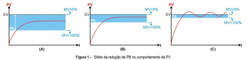
Figure 1- Effect of Pb reduction on PV behavior
In Figure 1.A, the process stabilizes with the large proportional band but far below the Setpoint. As the proportional band decreases (Figure 1.B), stabilization is closer to the Setpoint but too much reduction in the proportional band (Figure 1.C) can lead the process to instability (oscillation). Adjusting the proportional band is part of the process called “Control Tuning”.
When the desired condition (PV = SV) is reached, the proportional term results in MV = 0, i.e., no energy is delivered to the process, which causes the deviation to arise again. Therefore, a pure proportional control can never stabilize with PV = SV.
Many controllers that operate only in Proportional mode add a constant value to the MV output to ensure that, under the PV = SV condition, some energy is delivered to the system (Typically 50 %). This constant value is called Bias. When adjustable, it allows for PV stabilization closer to SV.
Including Integral Control – PI
The integral is not, by itself, a control technique since it cannot be employed separately from a proportional action. Integral action consists of a response at the controller output (MV), which is proportional to the amplitude and duration of the deviation. Integral action eliminates the deviation characteristic of strictly proportional control.
To better understand this, imagine a stabilized process with P control, as shown in Figure 2.A:
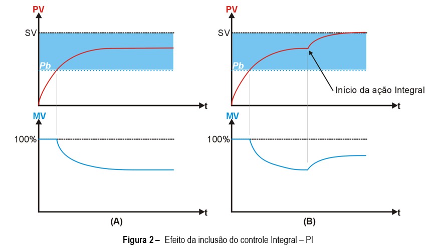
Figure 2 – Effect of including the Integral control − PI
In Figure 2.A, PV and MV reach an equilibrium condition where the amount of energy delivered to the system (MV) is what is needed to maintain PV at the value it is at. In this condition, if no disturbance occurs, the process will remain stable. Despite being stable, the process has not reached the Setpoint (SV), and there is a so-called “Steady-State Error”.
Now look at Figure 2.B, where, at the instant marked, the integral action has been included. Notice the gradual increase of the MV value and the consequent elimination of the Steady-State Error. Upon the inclusion of the integral action, the MV value is progressively changed to eliminate the PV error, until PV and MV reach a new equilibrium, but now with PV = SV.
The integral action works as follows: At regular intervals, the integral action corrects the MV value by adding the SV-PV deviation value to it. This action interval is called “Integral Time”, which can also be expressed by its inverse: Integral Rate (Ir). The Integral Rate (Ir) increases the integral performance in controlling the process.
The sole purpose of the integral action is to eliminate the Steady-State Error. When adopting an excessively active integral term, the process may become unstable. When adopting a low actuating integral, it delays too much the process to stabilize PV = SV.
>>> Read here about PID control tuning
Including Derivative Control – PD
The integral is not, by itself, a control technique since it cannot be employed separately from a proportional action. Derivative action consists of a response at the controller output (MV), proportional to the deviation variation rate. Derivative action slows the speed of PV variations, preventing them from rising or falling too quickly.
The derivative only acts when there is an error variation. If the process is stable, its effect is null. During disturbances or when starting the process, when the error is oscillating, the derivative always attenuates these variations, and therefore its main function is to improve the performance of the process during transients.
Figure 3 compares hypothetical responses of a process with P (A) and PD (B) control:
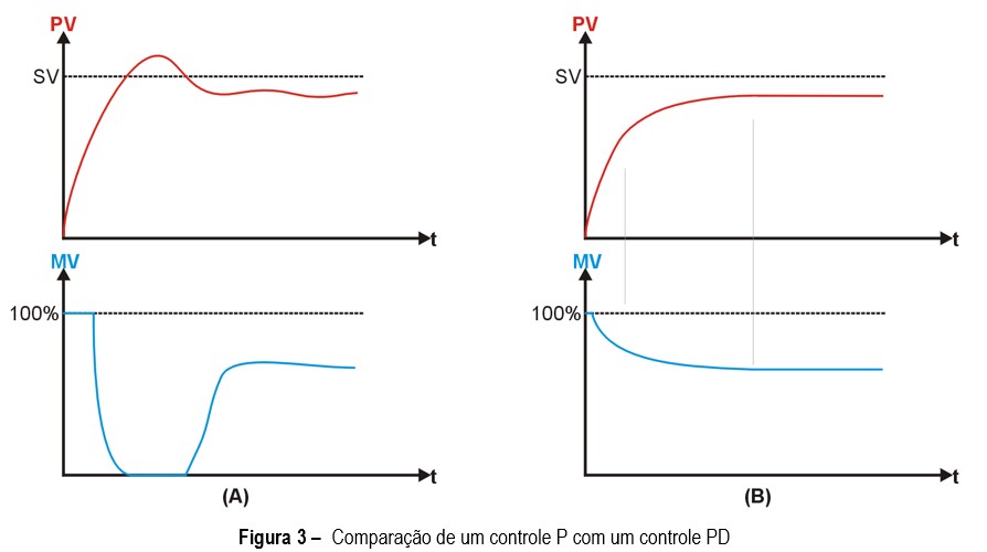
Figure 3 – Comparison of a P control with a PD control
In the P control (Figure 3.A), if the proportional band is small, it is likely that an overshoot occurs, where PV exceeds SV before it stabilizes. This is due to the long time that MV has been at its maximum value and because it has already started to decrease close to SV, when it is too late to prevent the overshoot.
One solution would be to increase the proportional band, but this would increase the Steady-State Error. Another solution is to include derivative control (Figure 3.B), which reduces the value of MV if PV is increasing too fast. By anticipating the PV variation, the derivative action reduces or eliminates overshoot and oscillations in the process transient period.
Mathematically, the derivative contribution to control is calculated as follows: At regular intervals, the controller calculates the variation of the process deviation and adds the value of this variation to MV. If PV is increasing, the deviation is reducing, resulting in a negative variation, which reduces the value of MV and consequently delays the increase of PV. The intensity of the derivative action is adjusted by varying the interval at which the difference is calculated. This parameter is called Derivative Time (Dt). Increasing the value of Dt increases the derivative action, reducing the rate of PV variation.
PID control
By joining the 3 techniques, we can unite the basic control of P with the error elimination of I and the oscillations reduction of D, but it creates difficulty to adjust the intensity of each term, a process called “PID Tuning.”
Process controller with PID Control: see all products
Read more:
7 reasons to choose a modular controller